Portfolio optimization using the efficient frontier and capital market line in Excel
Modern portfolio theory attempts to maximize the expected return of a portfolio for a certain level of risk. The theory is that by diversifying through a portfolio of assets we can get a higher return per unit of risk than we can by holding an individual asset, and that by adjusting the weights of each asset in a portfolio we can create an optimal portfolio for each investor’s level of risk aversion. Assuming that markets are efficient and that the assets in a portfolio aren’t perfectly correlated, we can reduce the total variance of a portfolio at any given expected return by combining assets in various weights.
Imagine a graph with risk on the X axis (measured as standard deviation of the asset’s historical returns) and dividend-adjusted return on the Y axis (measured as an average of historical return). We can plot every possible combination of risky assets in a portfolio to find the best possible return at each level of risk (and lowest possible risk for each level of expected return), and the resulting curve would have a higher return for any given level of risk than any individual asset. We can then combine our efficient portfolio with a risk free asset to create a portfolio of portfolios which we can graph as the capital market line. The capital market line will lie tangent to the efficient frontier at the portfolio with the highest sharpe ratio and represent the highest expected return per unit of risk; this represents the market portfolio. By levering up the capital market line or combining the optimized portfolio with a risk-free asset, we can achieve expected returns higher than the efficient frontier at respective standard deviations.
I will demonstrate how the efficient frontier and capital market line can be modeled in Excel in order to produce efficient portfolios. Let’s say that we choose to construct a risky portfolio with all 30 stocks in the Dow Jones Industrial Average. Below is a screenshot of the closing price of the stocks each month over the past five years, along with an index of the S&P 500 to include in our model.
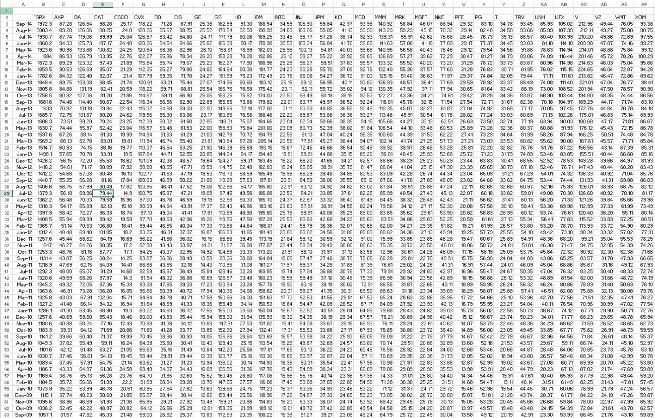
We can find continuously compounded monthly returns by taking the natural log of the closing price of each month / the closing price of the month prior. In Excel, this is entered as
=LN(Prices!B4/Prices!B5)
We create a table of continuously compounded monthly returns for the past five years, then compute the mean and standard deviation for each stock over this time horizon.
Covariance between returns on stocks is an important factor in this portfolio optimization because the value of diversification comes from assets that are not perfectly correlated; the greater the covariance, the more effectively we can diversify in order to reduce portfolio variability.
Covariance between returns on assets A and B is defined as
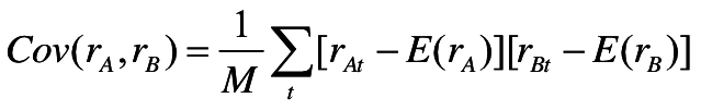
We must find the sum of every stock’s monthly change in price less its mean for the five-year monthly returns multiplied by every other stock’s monthly change in price less its mean for the five-year monthly returns. This number will then be divided by the number of months in our table. We can compute the covariance between every single stock in this model using matrix algebra - to do this we subtract the matrix of returns by the vector of means and multiply it by the transposed version of itself subtracted by the vector of means. In Excel, this is entered as
=MMULT(TRANSPOSE(B3:AF62-B64:AF64),B3:AF62-B64:AF64)/COUNT(A3:A62)
where the count command represents the number of monthly returns in my table.
The covariance table will appear as such:
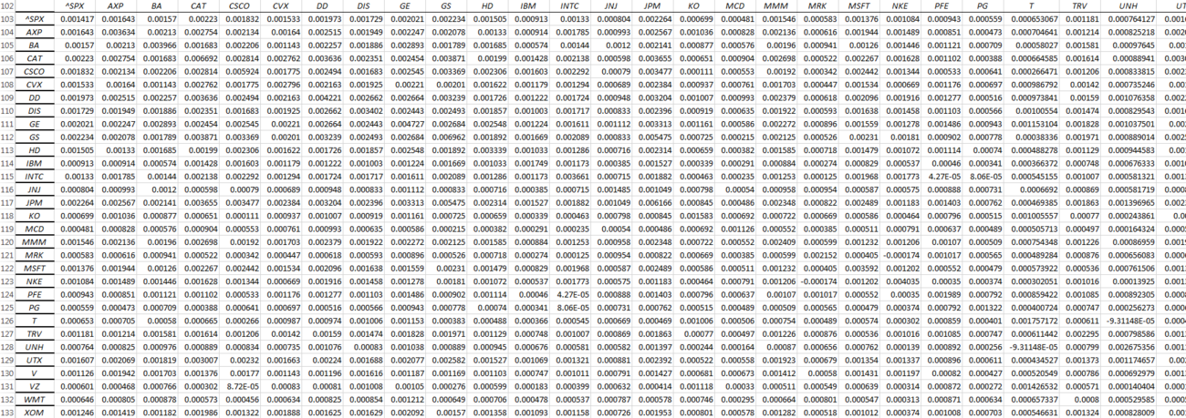
At this point we can construct a portfolio of arbitrary weights assigned to each stock. We then create cells to store the portfolio mean (vector of mean returns multiplied by vector of weights assigned to each stock to get a weighted average mean), portfolio variance (the vector of weights multiplied by the covariance matrix multiplied by the vector of weights), and portfolio standard deviation (square root of variance). Depending on the way I structure my spreadsheet, I may need to transpose vectors in order to multiply my matrices.
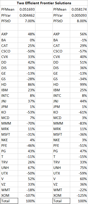
Upon constructing this part of the spreadsheet I can begin to find points on the efficient frontier. If we find two efficient portfolios, we can plot the entire efficient frontier by varying the weight of capital applied to each of these portfolios. I can use Excel’s Solver to find two efficient portfolios; the way I choose to do this is to maximize the value of the portfolio mean by changing the portfolio weights, subject to the constraint of the weights adding to 100% and a portfolio standard deviation of 7%. I then repeat the process for a constraint of portfolio standard deviation equal to 8%.
Allowing portfolio weights to be negative represents taking a short position in a stock.
I can copy and save the values of the portfolio weights, mean, variance, and standard deviation after each iteration of running Excel’s Solver to the side of my worksheet.
I can use a linear combination of my two efficient portfolios to effectively calculate the portfolio mean and standard deviation of every efficient combination of assets. I will arbitrarily pick a weight for one of my efficient portfolios within this new portfolio of portfolios and enter it into a cell in Excel, then find a weighted average return for my new portfolio. The covariance between these two efficient portfolios is defined as
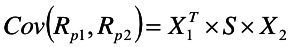
effectively multiplying the vector of weights for the first efficient portfolio by the covariance matrix of all stocks by the vector of weights for the second efficient portfolio. The standard deviation of the new portfolio of efficient portfolios will simply be the square root of this covariance.
At this point we can create a data table using Excel’s What-If Analysis to easily calculate the standard deviation and mean at many various weights of portfolio A with respect to portfolio B. The left column here represents the weight applied to my portfolio with standard deviation 7%, where the weight of my portfolio with standard deviation 8% equals 1 - portfolio of StDev 7%.
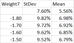
[Data table continues downward until Weight7 = 10]
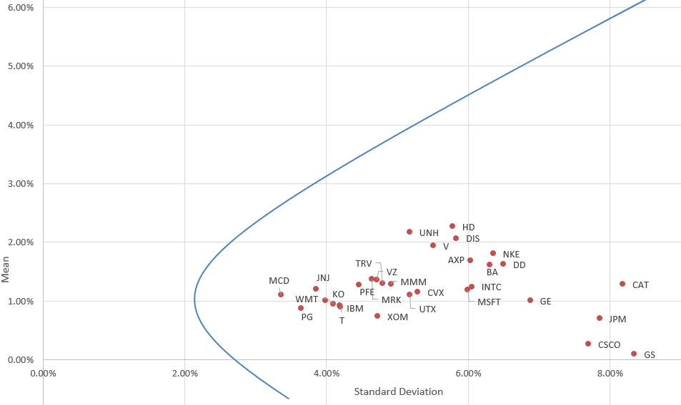
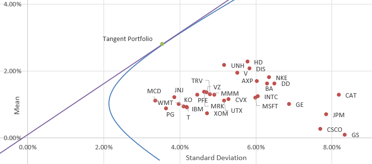
Plotting this data table as a scatterplot or scatter with smooth lines allows us to visualize the efficient frontier. Every point on the positively sloped region of this curve represents a portfolio that will offer the highest expected return per unit of risk.
This efficient frontier is computed based on two efficient portfolios, and if we were constructing a portfolio based on these findings we would be curious to see what weight to apply to each stock in this portfolio at any given point. This is easy to compute by creating a matrix with a column for each stock and a row for each weight of portfolio A used in the data table, then multiplying the weight of portfolio A by the respective weight of stock A in portfolio A and adding this to the weight of portfolio B (1 - weightA) multiplied by the respective weight of Stock A in portfolio B, and completing the entire matrix with such a formula. Alternatively, we can use Excel’s Solver to solve for our initial weight-seeking task with the constraint of a mean or standard deviation equal to a certain value to find the optimal portfolio weights at that efficient portfolio.
We can maximize the sharpe ratio [(portfolio mean - risk free rate) / portfolio standard deviation) to create a portfolio with the best historical risk-adjusted performance. The CAPM model allows us to combine the efficient portfolio with a risk-free asset to do attain a higher expected return than the efficient frontier. We do this by combining the risk free asset with the tangent portfolio containing all of our assets (this portfolio would represent the cap-weighted market portfolio). If we construct a portfolio at this point and keep the individual asset weights constant, we can lever up to reach a higher expected return or combine this portfolio with a risk free asset to a lower standard deviation; all the possible combinations of the risky portfolio and risk free asset make up the capital market line.
The CML’s slope is that of the sharpe ratio, thus indicating the best expected return per unit of risk, which will be superior to any portfolio on the efficient frontier. The CML also lies northwest of the efficient frontier, representing lower risk and/or higher expected return. The point of tangency represents a portfolio of 100% of the risky asset, whereas portfolios on the CML with a higher expected mean represent leverage and portfolios on the CML with a lower standard deviation combine the risky portfolio with a risk-free portfolio.
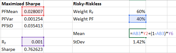
To model this in Excel, we first find the tangent portfolio by maximizing the sharpe ratio subject to the constraint of all portfolio weights adding up to 100% using Excel’s solver. We then construct a risky-riskless portfolio by combining the tangent portfolio with the risk-free asset in at an arbitrary weight. We find the mean and standard deviation of the portfolio at this arbitrary weight. Since the standard deviation of the risk-free asset is zero, we can simply multiply the tangent portfolio standard deviation by the tangent portfolio weight to find the standard deviation of the risky-riskless portfolio.
We can then create a data table as before.
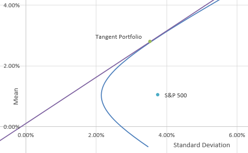
When graphed, this purple line represents the capital market line. Any rational investor would hold a portfolio of weights in proportions to the tangent portfolio constructed, then combine this portfolio with a risk-free asset according to their risk tolerance in order to generate expected returns above the efficient frontier.
The S&P 500 landed at the following spot for this data set.
Using such a model would help an investor who believes in efficient markets construct an optimal portfolio exposed to the highest expected return at the lowest variance. Limitations can be placed on this portfolio when using Excel’s solver if needed, for example to limit the maximum investment in any individual stock or disallow short selling.